My Matplotlib Cheatsheet (#1)

I find myself Googling the same matplotlib/pyplot queries over and over again. To make life easy, I started collecting some of them in a series of blog posts.
In this first post, I'll look at subplots and annotations.

Turn off axes

We can remove axes, ticks, borders, etc. with ax.axis('off'). This can be used to remove unnecessary subplots created with the subplots function from pyplot, for instance, when we only want to use the upper triangle of the grid. Here's an example:

	import matplotlib.pyplot as plt
	import numpy as np
	import scipy.stats as sts
	## create some random data
	n = 3
	Sigma = sts.wishart.rvs(scale=np.eye(n), df=n)
	xs = sts.multivariate_normal.rvs(cov=Sigma, size=1000)
	## plot histograms and scatter plots
	fig, axs = plt.subplots(n, n, figsize=(7,7))
	for i in range(n):
	for j in range(n):
	if i > j:
	axs[i, j].axis('off')
	elif i == j:
	axs[i, j].hist(xs[:, i], density=True)
	else:
	axs[i, j].scatter(xs[:, i], xs[:, j], s=5)
	fig.tight_layout()
	fig.savefig("axis-off.png", bbox_inches='tight', dpi=200)

view raw axis-off.py hosted with ❤ by GitHub

The result is:

Share axes between subplots after plotting

An alternative way of making a ragged array of subplots makes use of gridspec. The problem here is that it is a bit more difficult to share x and y axes. Of course add_subplot has keyword arguments sharex and sharey, but then we have to distinguish between the first and subsequent subplots. A better solution is the get_shared_x_axes() method. Here's an example:

	import matplotlib.pyplot as plt
	import numpy as np
	from matplotlib.gridspec import GridSpec
	## we want to make 23 plots using 5 columns
	n = 23
	ncols = 5
	## compute the required number of rows:
	nrows = n // ncols + 1 if n % ncols else 0
	## use gridspec to make the subplots
	fig = plt.figure(figsize=(7,7))
	gs = GridSpec(nrows, ncols)
	## reduce space between the subplots
	gs.update(wspace=0.07, hspace=0.07)
	## list will contain the subplots
	axs = []
	## some parameters for making our data
	u, v = 0.2, 0.3
	ts = np.linspace(0, 2*np.pi, 100)
	for i in range(n):
	## compute the row and column index
	col, row = i % ncols, i // ncols
	## and use gridspec to get a new subplot
	ax = fig.add_subplot(gs[row, col])
	## create some data and plot
	xs = (1+row) * (np.sin((col+1) * ts) + u * np.sin(ts))
	ys = (1+col) * (np.cos((row+1) * ts) + v * np.sin(ts))
	ax.plot(xs, ys, linewidth=3)
	## add the new subplot to the list
	axs.append(ax)
	## make y axis invisible
	if col > 0:
	ax.get_yaxis().set_visible(False)
	## make x axis invisible
	if row > 0:
	ax.get_xaxis().set_visible(False)
	else: ## move the x-ticks to the top
	ax.xaxis.set_ticks_position('top')
	## now we make the x and y axes shared and auto scale them
	axs[0].get_shared_x_axes().join(*axs)
	axs[0].autoscale(axis='x')
	axs[0].get_shared_y_axes().join(*axs)
	axs[0].autoscale(axis='y')
	fig.savefig("distorted-lissajous.png", bbox_inches='tight', dpi=200)

view raw share-axes.py hosted with ❤ by GitHub

The result is:

Hybrid (or blended) transforms for annotations

When you annotate a point in a plot, the location of the text is often relative to the data in one coordinate, but relative to the axis (e.g. in the middle) in the other. I used to do this with inverse transforms, but it turns out that there is a better way: the blended_transform_factory function from matplotlib.transforms.
Suppose that I want to annotate three points in three subplots. The arrows should point to these three points, and I want the text to be located above the point, but the text in the 3 subplots has to be vertically aligned.

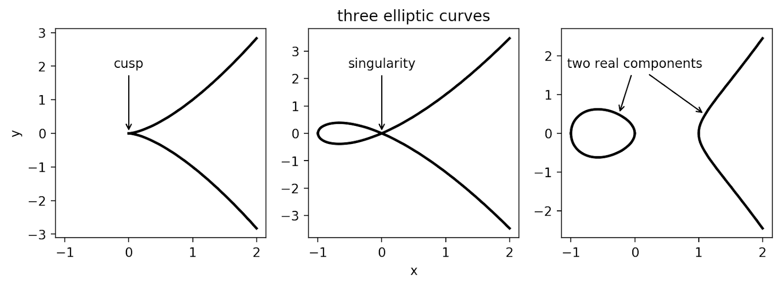
Notice that the y-axes are not shared between the subplots! To accomplish the alignment, we have to use the annotate method with a custom transform.

	import matplotlib.pyplot as plt
	import numpy as np
	## import the function we'll need for making the transforms
	from matplotlib.transforms import blended_transform_factory
	fig, axs = plt.subplots(1, 3, figsize=(10,3), sharex=True)
	fs = [
	lambda x: np.sqrt(x**3),
	lambda x: np.sqrt(x**2*(x+1)),
	lambda x: np.sqrt((x+1)*x*(x-1))
	]
	## plot some elliptic curves (the real part at least)
	xs = np.linspace(-1, 2, 1000)
	for f, a in zip(fs, axs):
	a.plot(xs, f(xs), color='k', linewidth=2)
	a.plot(xs, -f(xs), color='k', linewidth=2)
	def hybrid_trans(ax):
	"""
	This function returns a blended/hybrid
	transformation w.r.t. subplot ax.
	x-coord: use the data for positioning
	y-coord: use relative position w.r.t y-axis
	"""
	return blended_transform_factory(ax.transData, ax.transAxes)
	## avoid repetition: common key-word arguments for annotate
	kwargs = {
	"arrowprops" : {"arrowstyle": "->"},
	"ha" : "center",
	"va" : "bottom"
	}
	## give subplots names to avoid indexing
	ax, bx, cx = axs
	## the argument xytext determines where the text is positioned,
	## and we can pass a transformation with textcoords.
	## we'll use our custom "hybrid" transform so that the x-coord
	## corresponds to the data, and the y-coord is relative.
	ax.annotate("cusp", xy=(0,0), xytext=(0, 0.8),
	textcoords=hybrid_trans(ax), **kwargs)
	bx.annotate("singularity", xy=(0,0), xytext=(0, 0.8),
	textcoords=hybrid_trans(bx), **kwargs)
	## this is a bit of a hack: I want two annotate two points
	## with one text box. I'll make the second text box invisible
	## by setting alpha=0
	text = "two real components"
	xcoords = [-0.25, 1.1]
	alphas = [1, 0]
	for x, alpha in zip(xcoords, alphas):
	## use fs[2] to get the correct point
	cx.annotate(text, xy=(x,fs[2](x)), xytext=(0,0.8), alpha=alpha,
	textcoords=hybrid_trans(cx), **kwargs)
	## add some labels and titles...
	bx.set_xlabel("x")
	ax.set_ylabel("y")
	bx.set_title("three elliptic curves")
	fig.savefig("annotations.png", bbox_inches='tight', dpi=200)

view raw transform-annotate.py hosted with ❤ by GitHub

Using constant Stan functions for parameter array indices in ODE models

Stan's ODE solver has a fixed signature. The state, parameters and data has to be given as arrays. This can get confusing during development of a model, since parameters can change to constants (i.e. data), the number of parameters can change and even the state variables could change. Errors can easily creep in since the user has to correctly change all indices in the ODE function, and in (e.g.) the model block. A nice way to solve this is using constant functions. Constants in Stan are functions without an argument that return the constant value. For instance pi() returns 3.14159265... The user can define such constants in the functions block. Suppose that we want to fit the Lotka-Volterra model to data. The system of ODEs is given by $$\frac{dx}{dt} = ax - bxy\,,\quad \frac{dy}{dt} = cbxy - dy$$ and so we have a 2-dimenional state, and we need a parameter vector of length 4. In the function block, we will define a function int idx_a() { return 1; } that returns the index of the parameter $a$ in the parameter vector, and we define similar functions for the other parameters. The full model can be implemented in Stan as shown below. The data Preys and Predators is assumed to be Poisson-distributed with mean $Kx$ and $Ky$, respectively, for some large constant $K$. I fitted the model to some randomly generated data, which resulted in figure above.

	functions {
	// parameter indices
	int idx_a() { return 1; }
	int idx_b() { return 2; }
	int idx_c() { return 3; }
	int idx_d() { return 4; }
	// state indices
	int idx_x() { return 1; }
	int idx_y() { return 2; }
	// Lotka-Volterra ODEs
	real[] LV_sys(real t, real[] u, real[] par, real[] real_data, int[] int_data) {
	real du[2];
	// use index functions instead of integer literals
	du[idx_x()] = par[idx_a()] * u[idx_x()]
	- par[idx_b()] * u[idx_x()] * u[idx_y()];
	du[idx_y()] = par[idx_c()] * par[idx_b()] * u[idx_x()] * u[idx_y()]
	- par[idx_d()] * u[idx_y()];
	return du;
	}
	}
	data {
	int N;
	real Times[N];
	int Preys[N];
	int Predators[N];
	real K;
	}
	parameters {
	// initial conditions
	real<lower=0> x0;
	real<lower=0> y0;
	// parameters
	real<lower=0> a;
	real<lower=0> b;
	real<lower=0, upper=1> c;
	real<lower=0> d;
	}
	transformed parameters {
	real par[4];
	real u0[2];
	// again use index functions to make a parameter array
	par[idx_a()] = a;
	par[idx_b()] = b;
	par[idx_c()] = c;
	par[idx_d()] = d;
	// make an array for the initial condition
	u0[idx_x()] = x0;
	u0[idx_y()] = y0;
	}
	model {
	// integrate the ODEs
	real us[N, 2] = integrate_ode_rk45(LV_sys, u0, 0, Times, par, {0.0}, {0});
	// priors on the parameters
	x0 ~ normal(1, 1);
	y0 ~ normal(1, 1);
	a ~ normal(1, 1);
	b ~ normal(1, 1);
	c ~ beta(1, 1);
	d ~ normal(1, 1);
	// likelihood of the data
	Preys ~ poisson(to_array_1d(to_vector(us[:, idx_x()]) * K));
	Predators ~ poisson(to_array_1d(to_vector(us[:, idx_y()]) * K));
	}
	generated quantities {
	// export the solution of the ODE
	real us_hat[N, 2] = integrate_ode_rk45(LV_sys, u0, 0, Times, par, {0.0}, {0});
	// and simulate noise
	real us_sim[N, 2];
	for ( i in 1:N ) {
	for ( j in 1:2 ) {
	us_sim[i, j] = poisson_rng(us_hat[i, j] * K);
	}
	}
	}

view raw lotka-volterra.stan hosted with ❤ by GitHub

Of course, this is still a low-dimensional model with a small number of parameters, but I found that even in a simple model, defining parameter indices in this way keeps everything concise.
I used the following Python script to generate the data and interface with Stan.

	import numpy as np
	import matplotlib.pyplot as plt
	import pystan
	from scipy.integrate import solve_ivp
	from scipy.stats import poisson
	## choose nice parameter values
	a = 1
	b = 0.2
	c = 0.5
	d = 0.5
	## define the system
	def LV_sys(t, u):
	return [a*u[0] - b*u[0]*u[1], c*b*u[0]*u[1] - d*u[1]]
	## observation times and initial conditions
	N = 50
	Times = np.linspace(1, 25, N)
	x0 = 1
	y0 = 1
	u0 = [x0, y0]
	K = 10
	## generate random data
	sol = solve_ivp(LV_sys, (0, max(Times)), u0, t_eval=Times)
	Preys = [poisson.rvs(x*K) for x in sol.y[0]]
	Predators = [poisson.rvs(x*K) for x in sol.y[1]]
	## compile the Stan model
	sm = pystan.StanModel(file="lotka-volterra.stan")
	## prepare a data dictionary and initial parameter values for Stan
	data_dict = {
	'N' : N,
	'Times' : Times,
	'Preys' : Preys,
	'Predators' : Predators,
	'K' : K
	}
	def init_dict_gen():
	return {
	'a' : a,
	'b' : b,
	'c' : c,
	'd' : d,
	'x0' : x0,
	'y0' : y0
	}
	## sample from posterior
	sam = sm.sampling(data=data_dict, init=init_dict_gen, thin=10, chains=2, iter=5000)
	## make a figure with data and fit
	chain_dict = sam.extract(permuted=True)
	fig, ax = plt.subplots(1, 1, figsize=(7,5))
	ax.scatter(Times, Preys, color='tab:blue', edgecolors='k', zorder=2)
	ax.scatter(Times, Predators, color='tab:orange', edgecolors='k', zorder=2)
	pcts = [2.5, 97.5] ## percentiles
	colors = ['tab:blue', 'tab:orange']
	## plot trajectories
	for j, color in enumerate(colors):
	range_hat = [K*np.percentile(us, pcts) for us in chain_dict["us_hat"][:,:,j].T]
	ax.fill_between(Times, *np.array(range_hat).T, color=color,
	alpha=0.5, linewidth=0)
	## plot simulations
	for j, color in enumerate(colors):
	range_sim = [np.percentile(us, pcts) for us in chain_dict["us_sim"][:,:,j].T]
	ax.fill_between(Times, *np.array(range_sim).T, color=color,
	alpha=0.3, linewidth=0)
	ax.set_ylabel("Prey (blue), Predator (orange)\ndata and fit")
	ax.set_xlabel("Time")
	fig.savefig("LV-model-fit.png", bbox_inches='tight', dpi=200)
	## plot parameter estimates
	fig, ax = plt.subplots(1, 1, figsize=(7,3))
	parnames = ["a", "b", "c", "d", "x0", "y0"]
	real_par_vals = [a, b, c, d, x0, y0]
	## make violinplots of estimates
	pos = range(len(parnames))
	ax.violinplot([chain_dict[x] for x in parnames], pos)
	ax.set_xticks(pos)
	ax.set_xticklabels(parnames)
	## plot real parameter values
	ax.scatter(pos, real_par_vals, color='k')
	ax.set_ylabel("parameter estimate (blue)\nreal parameter value (black)")
	ax.set_xlabel("parameter name")
	fig.savefig("LV-model-estimates.png", bbox_inches='tight', dpi=200)

view raw lotka-volterra.py hosted with ❤ by GitHub

The following Figure show the parameter estimates together with the "real" parameter values